All my friends scattered to the wind after college and left Kansas City for other places in the country. Now, a few years after this diaspora, and a couple of children later, we talk about getting back together. There are arguments about what city has the best beer and the best weather, but still offers lots to do, and is relatively close to our families. No one city has the best of everything. A couple of our friends are moving to Portland and while it sounds pretty great, my wife gets a bit of the SAD if it’s too cloudy.
I thought I would find out for myself just how cloudy it really is. Wikipedia lists days of sunshine, but that seemed incomplete. Is it cloudy all day? Or is it cloudy in the morning like in San Francisco? This visualization is my attempt to quantify weather conditions and such. It’s probably not going to end any debates, but it’s a good start if weather is high on your list of must-haves before you move across the country.
Getting the data
The 2014 history data was scraped from the wunderground history api. You have to create an account, but it’s free up to 500 calls a day (per email, wink). Each response is a json blob of the daily summary and ~24 hourly observations with cloud cover, temperature, humidity, precipitation, etc. Here is a glossary of the terms in the response. I just scraped for the year of 2014, which corresponds to the black bars in the chart.
I found historical weather data from NOAA but it’s quite raw. Luckily, the University of Dayton has already done some of the heavy lifting for me (thanks, Ohio!). The Dayton data is broken down by a daily average temperature from 1995-2014 for many domestic and international cities, like so:
 1             1             1995         55.0
 1             2             1995         57.1
 1             3             1995         44.4
 1             4             1995         47.6
 1             5             1995         44.1
 1             6             1995         45.2
 1             7             1995         49.5
 1             8             1995         42.5
 1             9             1995         43.6
 1             10            1995         41.0
Preparing the data
Parsing the data was fairly straightforward. JavaScript isn’t a good language for scripting, but the functional programming features like map and reduce are really nice. We can eliminate some of the callback mess by using the someFuncSync() version of io methods, since we’re not creating a client-facing app. (please do not do this on a server). Not the most beautious code, but it got things moving.
Basically our goal is to create a list of averages per day. We’ll end up with
var fs = require('fs');

var files = {
    'CODENVER': 'denver',
    'NYNEWYOR': 'nyc',
    'CALOSANG': 'la',
    'ORPORTLA': 'portland',
    'ILCHICAG': 'chicago',
    'MOKANCTY': 'kc',
    'IEDUBLIN': 'dublin',
    'TUISTNBL': 'istanbul'
};

var finalData = {};

Object.keys(files).forEach(function (file) {

    var temps = [];
    // initialize array
    for (var i = 0; i < 12; i++) { temps[i] = []; }

    fs.readFileSync('weather_data/' + file + '.txt')
        .toString()
        .split('\n')
        .forEach(function (line, i) {
            var observation = line.trim().split(/\s+/);

            var date = new Date(observation[2], observation[0] - 1, observation[1]);
            var temp = observation[3] === '-99' ? null : parseFloat(observation[3], 10);

            // this might be confusing since we're representing dates as 0-indexed instead of the js convention of 1-indexed
            if (!temps[date.getMonth()][date.getDate() - 1]) temps[date.getMonth()][date.getDate() - 1] = [];
            temps[date.getMonth()][date.getDate() - 1].push(temp);
        });

    // clear out null values
    temps.forEach(function (month, monthIndex) {
        month.forEach(function (day, dayIndex) {
            var thisDay = day.filter(function (temp) {
                return temp;
            });

            temps[monthIndex][dayIndex] = {
                date: new Date(2014, monthIndex, dayIndex + 1),
                avgs: thisDay.sort(function (a, b) {
                    return a - b; // sort ascending
                }),
                max: Math.max.apply(Math, thisDay),
                min: Math.min.apply(Math, thisDay)
            };
        });
    });

    // transform temps back into a flat array of dates
    var finalTemps = temps.reduce(function (memo, monthly) {
        return memo.concat(monthly);
    });

    // splice out leap day
    finalTemps.splice(59, 1);

    finalData[files[file]] = finalTemps;

    console.log('created finalData[' + files[file] + ']');

});

fs.writeFileSync('averages.json', JSON.stringify(finalData));
Many of the architecture (using that word loosely) decisions for this project are guided by the fact that while d3 can do many awesome stats things, you have to consider file download size. I definitely could have piped all these files directly to the browser and probably written less lines of code overall, but the 2014 data for ONE city is 27mb. That being said, this could be pretty intresting if set up as a service with some of the node.js streaming tools parsing the JSON and an upgraded account from wunderground.
Making the chart
If you haven’t tried d3 yet, it’s time to take the plunge. Basically, this is a glorified bar chart where the bars don’t end at 0, but go from a high to a low temperature. Here are some of the intresting bits:
// setting x and y scales.
// the x domain is hard-coded to 2014, but it doesn't really matter, I just picked a year with no leap year.
var x = d3.time.scale()
    .domain([new Date(2014, 0, 1), new Date(2014, 11, 31)])
    .range([0, width]);
// start at 0° and end at 100°F
var y = d3.scale.linear().domain([0, 100]).range([height, 0]);
d3 has some nice stats stuff built in, just make sure to check first before you try to write your own methods. I wanted to show the interquartile range for the historical average temperatures, and d3 has quantile methods.
// draw inner quartile
svg.selectAll('.quart')
    .data(averages[initCity])
    .enter().append('rect')
        .attr('class', 'quart')
        .attr('x', function (d) { return x(d.date); })
        .attr('y', function (d) { return y(d3.quantile(d.avgs, 0.75)); })
        .attr('width', barWidth)
        .attr('height', function (d) {
            return height - y(d3.quantile(d.avgs, 0.75) - d3.quantile(d.avgs, 0.25));
        })
        .attr('fill', centerColor);
I had trouble getting the months to show up as ticks on the x-axis, but here’s what I ended up with:
var xAxis = d3.svg.axis()
    .scale(x)
    .orient('bottom')
    .ticks(d3.time.months)
    .tickFormat(d3.time.format('%B'));

// later...
svg.append('g') // x axis
    .attr('class', 'x axis') // this is so you can style the svg elements with css
    .attr('transform', 'translate(0,' + y(0) + ')') // cross @ 0
    .call(xAxis)
    .selectAll('.tick text')
        .style('text-anchor', 'start')
        .attr('transform', 'rotate(45)') // rotate so labels fit on mobile
        .attr('x', 6)
        .attr('y', 6);
Refining the chart
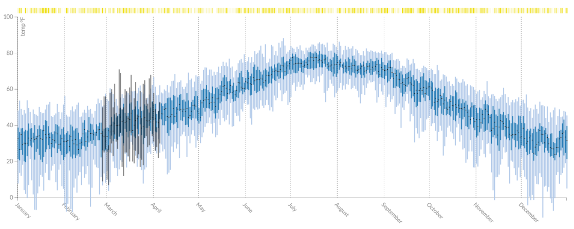
I wanted to compare 2014’s temperatures to the running average, but overlaying all the data made the chart too busy. I tried different colors and opacities, and in the end I settled on a mouse-driven interaction, where you can see 20 days at a time. This still gives you a sense of what the year was like without overwhelming the rest of the data.
Showing the sunshine as a percentage was pretty fun. The measurements are from 2014, so I have the hourly condition measurements. Conditions can be something like “cloudy”, “snow”, or “brimstone”, etc. I have the daily list of 24 observations, and made the yellow bar more translucent the more cloudy it was. I counted the conditions “clear”, “sunny”, “scattered clouds”, “partly cloudy” (I’m a glass-half-full sort of guy) and “mostly sunny” as clear-ish. So if it was snowing for half the day and clear for the other half, the yellow bar would be at 0.5 opacity.
Finally
It’s the middle of the winter here in nyc, and LA looks pretty great after building this chart. And to answer the original question, yes, it really is that cloudy in Portland.